
PDF chapter test TRY NOW
We will see a few cases which can elaborate on the relation between time and distance.
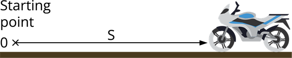
The above figure shows a bike travelling along a straight line away from the starting point \(O\) with uniform speed.
The distance of the bike is measured for every second. The distance and time are recorded, and a graph is plotted using the data. The below graph shows the possible results of the journey.
Case I: If the bike staying at rest, then the distance is constant for every second.
| Time(\(s\)) | \(0\) | \(1\) | \(2\) | \(3\) | \(4\) | \(5\) |
| Distances(\(m\)) | \(0\) | \(20\) | \(20\) | \(20\) | \(20\) | \(20\) |
If we plot a graph for the constant distance, we get a straight line, as shown in the below graph.

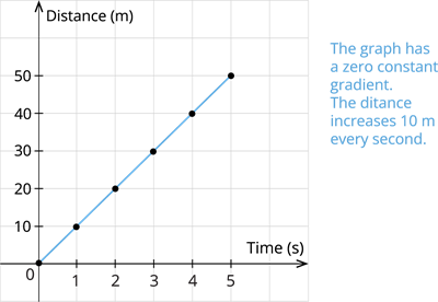
Case II: The bike travelling at a uniform speed of \(10\) \(\frac{m}{s}\)
| Time(\(s\)) | \(0\) | \(1\) | \(2\) | \(3\) | \(4\) | \(5\) |
| Distances(\(m\)) | \(0\) | \(10\) | \(20\) | \(30\) | \(40\) | \(50\) |
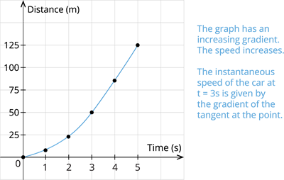
Case III: The bike travelling at increasing speed.
| Time(\(s\)) | \(0\) | \(1\) | \(2\) | \(3\) | \(4\) | \(5\) |
| Distances(\(m\)) | \(0\) | \(5\) | \(20\) | \(45\) | \(80\) | \(125\) |
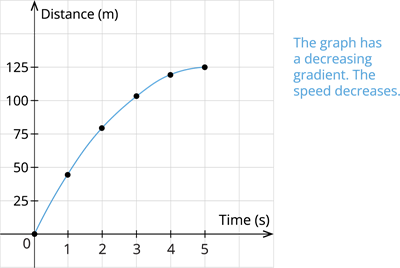
Case IV: The bike travelling at decreasing speed.
| Time(\(s\)) | \(0\) | \(1\) | \(2\) | \(3\) | \(4\) | \(5\) |
| Distances(\(m\)) | \(0\) | \(45\) | \(80\) | \(105\) | \(120\) | \(125\) |
 Register for free to see more content